The purpose of this document is to provide a description of the work I have done fitting showers using a maximum likelihood method. If you don't know what the method of maximum likelihood is, you should learn. You can find it it any good statistics book.
All results presented here use the "old" calibration constants produced by Tony.
Any references to "offline" code refer to the code in /disk02/Milagro/analysis/offline.
I begin with the assumption that the current offline angle fitter for the most part produces reasonable results if the PE cut is chosen to be 1.5 or greater. I use a PE cut of 2 in the analysis.
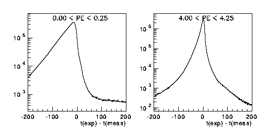
I reconstructed 20,000,000 showers offline and histogramed the residuals (time_expected-time_measured) by the number of PE's detected by the tube. Figure 1 shows the 2 residual plots, for two different PE ranges. I chose a quarter PE as the range covered by each plot. Certainly this is much better than our resolution justifies, but the computer does the work, not me. I go all the way up to 50 PE's and assume anything larger has the same timing distribution as a 50 PE hit.

I smoothed the 200 probability distribution histograms and wrote the contents of each bin to a file.
My Angle fitting software reads in the histograms files, and normalizes the contents and take the log. I then use a modified version of the numerical recipes routine SPLINE to calculate the second derivative of the function that connects the histogram bins at the center of each bin. With the value at each bin center and the second derivative also know it is a simple matter to perform a cubic spline interpolation and generate a function that has the shape of the histograms and is continuous in the its first and second derivatives. The continuity in the derivatives is important for the numerical fitting process.
I now have a functional form for the log probability distributions for a tube of any pulse height. So, for any hypothetical (theta,phi,time) generate the probability for each tube. The "likelihood" that the measured tube hit times were produced by a shower of a given (theta,phi,time) is maximized to get the best estimate of the shower angle.
I use as starting positions the shower results from the offline shower fitter.
The first thing the one notices is that my fitter converges for about 98% of showers compared to 89% for the offline. The theta distribtions for the two fitters are shown in figure 2.
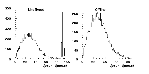
The showers that fail the offline fitter, but pass mine are mostly reconstructed with theta near 90 deg. The guys that reconstruct at 90 deg are probably muons, but they are not necessarily muons at 90 deg. Simulated muons events with angles smaller than 90 deg are often reconstructed to be at 90 deg.
Figure 3 shows the DelEO distribution for showers that produce a DelEO
for both fitting methods. 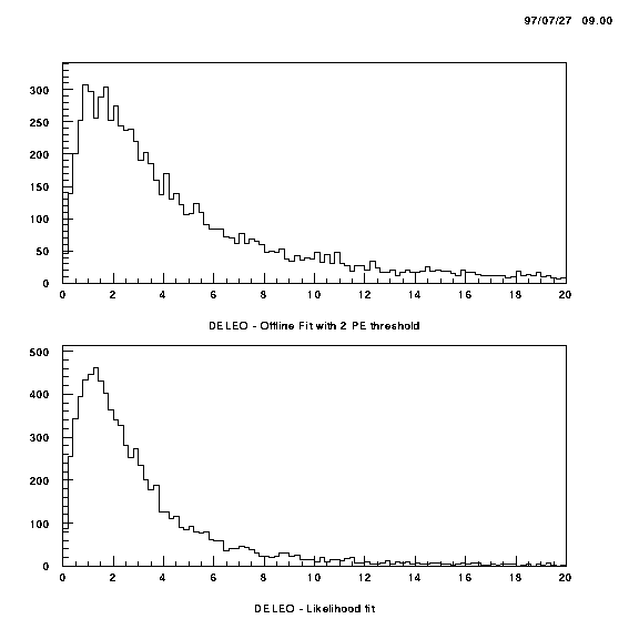
In this comparison, the offline DelEO is much larger than the DelEO produced by my fitter.
The last figure is a plot of the average value of DelEO for showers that produce a DelEO for both fitters plotted as a function of PE cut.
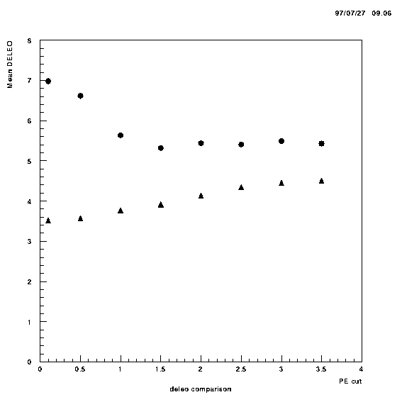
The circles are the offline DelEO means, and the triangles are the means for my fitter. As has been observed before by myself and others, the best PE cut for the offline code is at about 1.5 to 2.0 PEs. But, for my fitter the introduction of a PE cut always makes the DelEO worse.
The problem with this method is that it run at about 25Hz on our SGI O2s. Kahuna is only 5 times faster than the O2s at most, so this code runs too slow to keep up with the data taking. I have some ideas how to make the code faster, but they have not yet been tried.
For those who wish to try my code, e-mail me for the source.