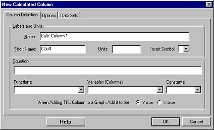
This feature allows you to create a new column of data for further analysis. This column can be mathematically related to another column or columns. For example, if you have current and voltage data, you can use a new column to calculate current times voltage or power. You can also use extra columns to show the relationships between variables.

Name: The long name is used in graph axis labels, column headings
and menus whenever there is sufficient room. You cannot use a quotation
character () in the Long Name
Short Name: The short name is used in graph axis labels, column headings and menus whenever there is limited room. If you do not enter a Short Name, the first letter of the Long Name will be used.
Units: The unit name follows the column name in graph axis labels and column headings. If the units that you enter are not the same as a visible line on the active graph window, you will be warned that your column will not be automatically shown in the graph. You can either re-enter units that match a visible line, or click on the Y-axis label in the graph window and select your column to be drawn.
You can choose special symbols to be included in all of the above
fields. Macintosh users can insert symbols by holding down the Option key
and pressing:
p for p
m for m
0
for o
shift and = for
+
Note: There are
several symbols, and some also vary from font to font. The Key Caps program
can be used to see all available symbols. Key Caps is a program that
comes with the MacOS system software.
| Equation: | This box contains the formula used to calculate the new column. Insert from the fields below. |
| Variables (Columns): | This provides access to a list of the other columns. The columns you select will be copied to the Column Definition. |
| Functions: | The functions available in the New Column and Edit Column Definition dialog boxes are: |
- Trigonometric functions will use degrees or radians as set in About [file name] on the File menu.
- For more information about Savitsky-Golay methods see Numerical
Recipes in C:
http://lib-www.lanl.gov/numerical/bookcpdf.html
chapter 15
|
|
|
|
|
The abs() function takes the absolute value of a cell. |
|
|
Arccosine function. The arccosine(X) calculates the angle whose cosine equals X. X should always be between 1 and 1. |
|
|
Arcsine function. The arcsine(x) calculates the angle (in radians) whose sine equals x. X should always be between 1 anArcsine function. The arcsine(X) calculates the angle whose sine equals X. X should always be between 1 and 1. |
|
|
The arctangent(X) calculates the angle whose tangent equals X. |
|
|
ceiling("X") returns a column of values where each value is the smallest integer greater than or equal to X. |
|
|
constant(x, num) cretaes a column with num rows of the value x. num can either be a real number or a column, and refer to a specific data set. If num is a column, then the size of that column is used to determine how many rows to create. |
|
|
Cosine function. |
|
|
This function returns the difference between the current data point and the next. |
|
|
derivative("Y", "X") returns the numerical derivative of "Y" with respect to "X". The numerical derivative is the weighted average of the slope of points N points around each point. You can set N in File:Settings. This is the fastest way to calculate derivatives. |
|
|
derivativeSG("Y", "X") returns the Savitsky-Golay derivative of "Y" with respect to "X". A polynomial is fitted to N points around each point and the derivative of that polynomial is used. N may be set in File:Settings. This is very accurate but can be slower than other methods. |
|
|
exp("X") will return a column of values e^X, where e is The base of the natural logarithm, 2.718281828. |
|
|
floor("X") for each value in X, floor returns the smallest integer less than or equal to that value. |
|
|
integral("Y","X") creates a column where the n'th row = sum (Yi + Yi-1)/2 * (Xi-Xi-1) for i = 1 to n. This is the integral using the midpoint rule. |
|
|
Natural logarithm. The inverse function of exp( ). |
|
|
logarithm (base ten) |
|
|
max("X") returns the largest value in X. (It will only return 1 value -- not another column the way most functions do.) |
|
|
mean("X") returns the average value of X. if there are n values then the average is (x1 + x2 + ... + Xn) / n. (It will only return 1 value -- not another column the way most functions do.) |
|
|
median("X") returns the "middle" value of X. Half the values in X will be greater than or equal to the median, and half the values will be less than or equal to the median. (It will only return 1 value -- not another column the way most functions do.) |
|
|
min("X") returns the smallest value in X. (It will only return 1 value -- not another column the way most functions do.) |
|
|
noise(k, "X"): Returns Gaussian noise of amplitude k ("X" is used to determine the number of points in the returned column). Num can either be a real number or a column. |
|
|
NumRows("X") returns the number of values in "X". (It will only return 1 value -- not another column the way most functions do.) |
|
|
randInt(min, max, num): Creates a column of num rows where each value is a random integer between min and max (inclusive). Num can either be a real number or a column. |
|
|
randReal(min, max, num): Creates a column of num rows where each value is a random real number between min and max (inclusive). Num can either be a real number or a column. |
|
|
round("X") returns a column of values where each value is X rounded to the nearest integer (rounding 0.1 gives 0, 0.6 gives 1). |
|
|
secondDerivative("Y", "X") takes two columns and returns the numerical second derivative of "Y" with respect to "X". If you leave out the second argument, the first column in the data set will be used. This function just calls the function derivative twice (see description of derivative). |
|
|
secondDerivativeSG("Y", "X") returns the Savitsky-Golay second derivative of "Y" with respect to "X". A polynomial is fitted to N points around each point and the second derivative of that polynomial is used. N may be set in File:Settings. This is very accurate but can be slower than other methods. |
|
|
Sine function. |
|
|
SmoothAve("X") takes a column and returns weighted averages (closer points are weighted higher). For each point, N points around that point are used in the averaging. You can set N in File:Settings. This is very fast and works well for linear data, but will always flatten and widen areas around local minimums or maximums. |
|
|
SmoothSG("Y","X") returns the Savitsky-Golay smoothed "Y" values. A polynomial is fitted to N points around each point and the value of that polynomial is used. N may be set in File:Settings. "X" is used to help the polynomial fit. This gives a very nice smoothed line that preserves local minimums and maximums but can be slower than other methods. If you leave out the second argument, the first column in the data set will be used. |
|
|
Square root |
|
|
Standard deviation |
|
|
sum() Sum takes a column, "X", as its argument and returns the sum of the numbers. |
|
|
Tangent function. |
|
|
DerivativeTimeShift ("Y", "X"): returns the derivative of "Y" with respect to "X". This function is specifically designed to be used with photogate and picket fence data. The derivatives returned are adjusted to estimate values at the start of the timing interval, instead of the midpoint. For details see The Physics Teacher, Vol 35, April 1997, p.220. |
You must specify the dependent column but the independent column is optional. If the independent variable is left out, the derivative of the dependent variable is taken with respect to the first column in the data set.
If data is imported from an experiment file, you may want to specify
the independent column. For example, if the imported data included time
in the first column but you wanted to calculate the derivative of pH with
respect to volume, you have to define the derivative as derivative("pH","Volume").
Constants:
|
|
|
|
|
3.14159265359. The ratio of a circle's circumference to its diameter. |
|
|
2.718281828. The base of the natural logarithm, ln( ) |
Select which axis you wish the new column to be added to by clicking the X-Axis or Y-Axis radio buttons.
You can edit the columns by either double-clicking the column name in
the Data Browser or choosing
Column
Options from the Data Menu.
See Also: