 Click here for the
  Displayed above are graphs of the five Legendre polynomials,
Pn(x) over the interval -1≤x≤1 for n=1,2,3,4 and 5.
These functions are orthonormal with respect to the standard inner
product. For further details see
Displayed above are graphs of the five Legendre polynomials,
Pn(x) over the interval -1≤x≤1 for n=1,2,3,4 and 5.
These functions are orthonormal with respect to the standard inner
product. For further details see
 For further details see
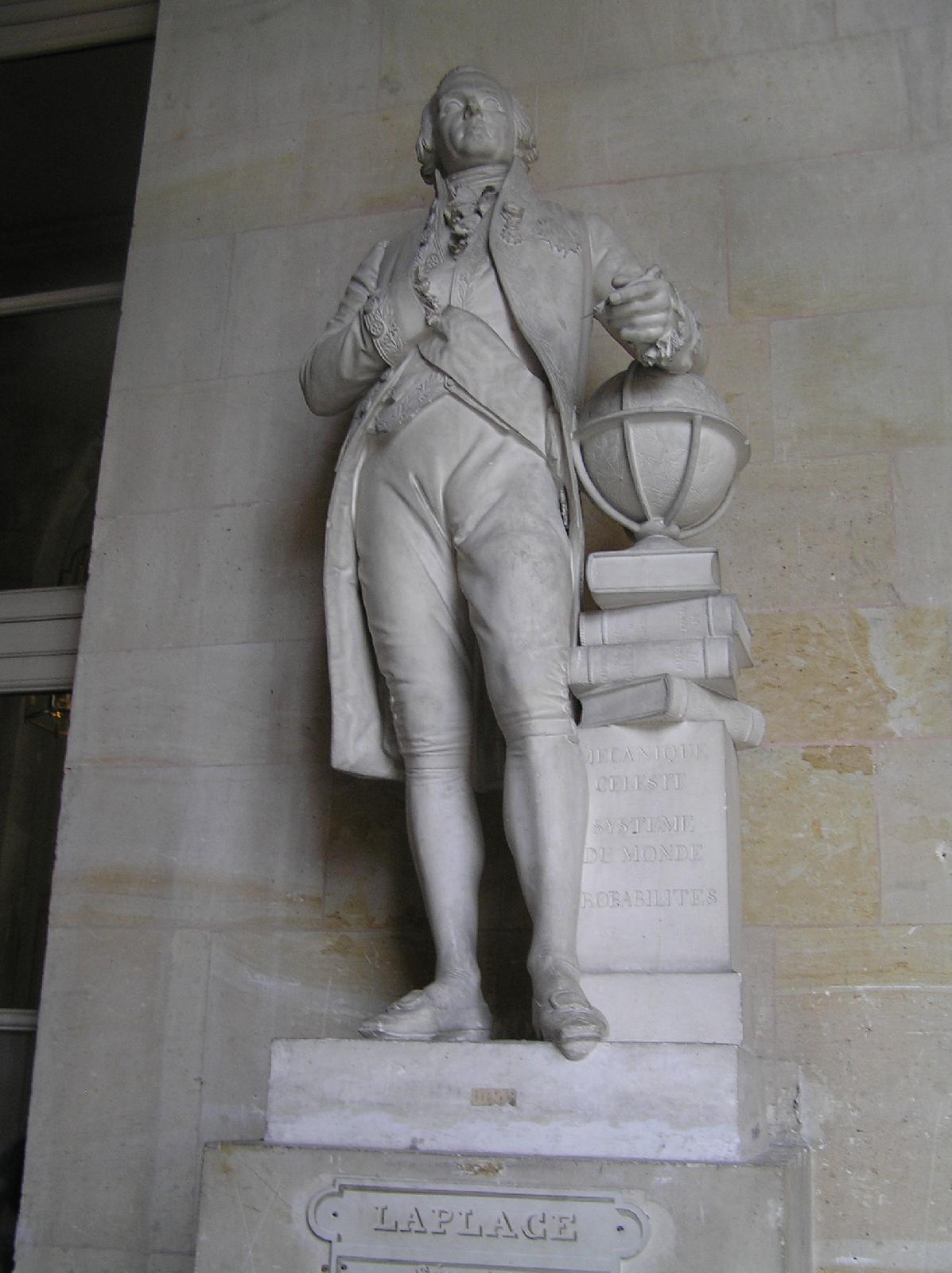 In June, 2012, when I was visiting the (newly restored) Palace of Versailles, located 10 miles
west-southwest of Paris, I came across a statue of Pierre-Simon Laplace
(1749--1827). He is among the few scientists honored at the Palace.
In June, 2012, when I was visiting the (newly restored) Palace of Versailles, located 10 miles
west-southwest of Paris, I came across a statue of Pierre-Simon Laplace
(1749--1827). He is among the few scientists honored at the Palace.

This page contains all class handouts and other items of interest for students of Physics 116C at the University of California, Santa Cruz.
SPECIAL ANNOUNCEMENTS
Letter grades are based on the cumulative course average, which
is weighted according to:
homework (9 problem sets with the low score dropped)---40%;
midterm exam---25%; and
the final exam---35%. This cumulative course average is then
converted into a letter grade according to the following
approximate numerical ranges:
A+ (92--100); A (83--92); A- (77--83); B+ (71--77); B (65--71);
B- (59--65); C+ (53--59); C(47--53); D(41--47); F (0--41).
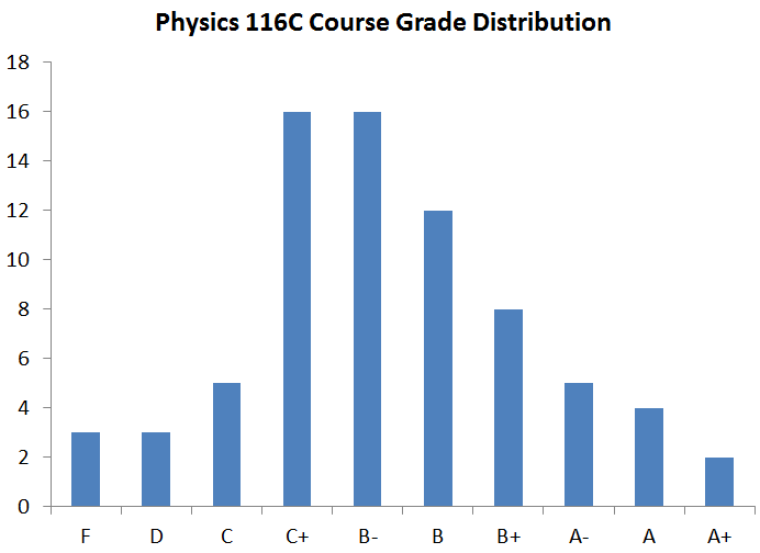
Here is the statistical summary of the distribution of
the cumulative course averages:
mean: 63.6
median: 61.7
standard deviation: 12.8
high: 96.9
low : 38.2
Students who did not take the final exam are not included in this
statistical summary.
Solutions to the final exam (and a link to the final exam statistics) can be found in Section VI on this website.
Physics 116C: Mathematical Methods in Physics III
I. General Information and Syllabus
The General Information and Syllabus handout is available
in either PDF or Postscript format
[PDF | Postscript]
Some of the information in this handout is reproduced below.
Class Hours
Lectures: Tuesdays and Thursdays, 12--1:45 pm, Physical Sciences
Building, Room 110
Discussion Section
Mondays 5:00--6:10 pm, Natural Sciences Annex, Room 101
Instructor Office Hours
Mondays, 2:30--4:30 pm.
I will also be available for consultation after class on Tuesdays
and Thursdays.
Required Textbook
Mathematical Methods in the Physical Sciences, by Mary L. Boas
The latest list of errata for the textbook is available in the following PDF file.
Course Grading and Requirements
40% Weekly Homework (9 problem sets)
25% Midterm Exam (Thursday, November 8, 2012, 12--1:45 pm)
35% Final Exam (Thursday, December 13, 2012, 12--3 pm)
Homework assignments will be posted on the course website on a weekly basis, and are due at the beginning of class on the due date specified on the assignment sheet. The homework problem sets are not optional. You are encouraged to discuss the class material and homework problems with your classmates and to work in groups, but all submitted problems should represent your own work and understanding. In order that homework can be graded efficiently and returned quickly, there will be a 50% penalty for late homework. This penalty may be waived in special circumstances if you see me before the original due date. Homework solutions will be posted to the course website one or two days after the official due date; no late homeworks will be accepted after that.
There will be one midterm exam and one final exam:
- Thursday November 8, 2012 12--1:45 pm Midterm exam
- Thursday December 13, 2012 12--3 pm Final exam
Course Syllabus for Physics 116C
A snapshot of the course lecture schedule appears below.
The dates given below are approximate.
Brief Course Outline for Physics 116C |
||
|---|---|---|
| TOPIC | Lecture dates | Readings | Series solutions of differential equations | Sept 27 | Boas Chapter 12, sections 1, 11, 21 | Legendre polynomials and functions | Oct 2, 4, 9 | Boas, Chapter 12, sections 2--10 | Bessel functions | Oct 9, 11, 16 | Boas, Chapter 12, sections 12--18, 20 | The Sturm-Liouville problem | Oct 18 | Boas, Chapter 12, section 23 | Hermite and Laguerre functions and polynomials | Oct 23 | Boas, Chapter 12, section 22 | Partial differential equations of mathematical physics | Oct 25, 30 | Boas, Chapter 13, sections 1--4 | Problems with cylindrical and spherical symmetry | Nov 1, 6 | Boas, Chapter 13, sections 5--7 | MIDTERM EXAM | Nov 8 | September/October lectures | Potential theory and Green function techniques | Nov 13 | Boas Chapter 13, section 8 | Integral transform solutions of partial differential equations | Nov 15 | Boas Chapter 13, section 9 | Theory of probability | Nov 20, 27 | Boas Chapter 15, sections 1--4 | Random variables and probability distributions | Nov 29, Dec 4 | Boas Chapter 15, sections 5--9 | Statistics and experimental measurements | Dec 6 | Boas Chapter 15, section 10 | FIANL EXAM | Dec 13 | entire course material |
A summary of the course syllabi for Physics 116A,B,C is available in either
PDF or Postscript format
[PDF | Postscript]
II. Learning Support Services
Learning Support Services (LSS) offers course-specific tutoring that is
available to all UCSC students. Students meet in small groups (up to 4
people per group) led by a tutor. Students are eligible for up to
one-hour of tutoring per week per course, and may
sign-up for tutoring
beginning October 9th at 10:00am.
III. Computer algebra systems
Although the use of computer algebra is not mandatory in this class, it can be a very effective tool for pedagogy. In addition, if used correctly, it can be an invaluable problem solving tool. Two of the best computer algebra systems available are Mathematica and Maple. Another useful software system for applied mathematics is MATLAB, which provides a high-level language and interactive environment for numerical computation, visualization, and programming.There are student versions of Mathematica, Maple and MATLAB available, which sell for the cost of a typical mathematical physics textbook. If you do not wish to invest any money at this time, you can use Mathematica and MATLAB for free at computer labs on campus. For further information click here. A complete list of all the software available in the Learning Technologies computer labs, along with the file path to find the programs on each workstation can be found at this link.
IV. Homework Problem Sets and Exams
Problem sets and exams are available in either PDF or Postscript format.
- Homework Set #1--due: Tuesday October 9, 2012 [PDF | Postscript]
- Homework Set #2--due: Tuesday October 16, 2012 [PDF | Postscript]
- Homework Set #3--due: Tuesday October 23, 2012 [PDF | Postscript]
- Homework Set #4--due: Tuesday October 30, 2012 [PDF | Postscript]
- Homework Set #5--due: Tuesday November 6, 2012 [PDF | Postscript]
- Midterm Exam---Thursday November 8, 2012 [PDF | Postscript]
- Homework Set #6--due: Thursday November 15, 2012 [PDF | Postscript]
- Homework Set #7--due: Tuesday November 27, 2012 [PDF | Postscript]
- Homework Set #8--due: Tuesday December 4, 2012 [PDF | Postscript]
- Homework Set #9--due: Tuesday December 11, 2012 [PDF | Postscript]
- Final Exam---Thursday December 13, 2012 [PDF | Postscript]
V. Practice Problems for the Midterm and Final Exams and their solutions
Practice midterm and final exams can be found here. These should give you some idea as to the format and level of difficulty of the exam. Also provided are additional practice problems to aid you in your preparation for the exams. Solutions to the practice exam and additional practice problems will be provided two days before the corresponding exam.
- Additional practice problems #1 [PDF | Postscript] and their solutions [PDF | Postscript]
- Practice Midterm Exam [PDF | Postscript] and their solutions [PDF | Postscript]
- Additional practice problems #2 [PDF | Postscript] and their solutions [PDF | Postscript]
- Practice Final Exam [PDF | Postscript] and their solutions [PDF | Postscript]
VI. Solutions to Homework Problem Sets and Exams
The homework set and exam solutions are available in either PDF or postscript format. Solutions will be posted one or two days after the homework is due and after the exams have been completed. Solutions to homework sets are provided by Angelo Monteux, with some further editing by Howard Haber. There is no password required to view the solutions.
- Solution Set #1 [PDF | Postscript]
- Solution Set #2 [PDF | Postscript]
- Solution Set #3 [PDF | Postscript]
- Solution Set #4 [PDF | Postscript]
- Solution Set #5 [PDF | Postscript]
- Solutions to Midterm Exam [PDF | Postscript] [exam statistics]
- Solution Set #6 [PDF | Postscript]
- Solution Set #7 [PDF | Postscript]
- Solution Set #8 [PDF | Postscript]
- Solution Set #9 [PDF | Postscript]
- Solutions to Final Exam [PDF | Postscript] [exam statistics]
VII. Other Class Handouts
1. The Wronskian is especially useful in the theory of ordinary linear differential equations. If y1(x), y2(x),..., yn(x) are linearly independent solutions to the differential equation, then their Wronskian is nonvanishing. Even if the solutions cannot be determined analytically, one can determine the Wronskian using Abel's formula. This formula is derived in this handout entitled Applications of the Wronskian to ordinary linear differential equations, and a number of other applications of the Wronskian are exhibited. [PDF | Postscript].
2. Given a homogeneous second-order linear differential equation, one can determine whether a given point (such as the origin) is an ordinary point, a regular singular point or an irregular singular point. In the first case, one can determine a power series solution to the differential equation. In the second case, the Frobenius method can be applied (which yields a generalized power series solution). The irregular singular point is not amenable to either method. [PDF | Postscript].
3. An optional handout entitled Series solutions to a second order linear differential equation with regular singular points provides details on how to evaluate the corresponding series and determine the two linearly independent solutions. In particular, if the roots of the indicial equation are equal, then one of the linearly independent solutions includes a logarithmic term. The logarithmic case can also arise if the roots of the indicial equation differ by an integer. After providing the general formulae for the various cases, a number of simple examples are given where the second linearly independent solution contains a logarithm. One appendix of this handout employs the Bessel differential equation to illustrate all the possible cases. [PDF | Postscript].
4. The function (1-2xt+t2)-1/2 is the generating function for the Legendre polynomials. An explicit proof of this result is presented by constructing the Taylor series for (1-2xt+t2)-1/2 around t=0 and extracting the coefficient of tn. Some applications of the generating function are given. [PDF | Postscript].
5. The Laplace and Poisson equations, subject to Dirichlet, Neumann, or mixed boundary conditions, are well-posed problems. In particular, the solution to these problems, if they exist, are unique (or in the Neumann case, unique up to an arbitrary additive constant). The proof of this latter statement is provided in the class handout entitled Uniqueness of solutions to the Laplace and Poisson equations. [PDF | Postscript].
6. In solving linear second order partial differential equations subject to Dirichlet, Neumann or mixed boundary conditions, one can sometimes express the general solution to the partial differential equation as some kind of Fourier series prior to imposing the last boundary condition. The coefficients of that series are then determined uniquely once the final boundary condition is imposed. In a class handout entitled Various kinds of Fourier series, I have summarized the properties of five different kinds of Fourier series that can arise in practical problems. The Fourier series can involve only sines or only cosines, or it may contain both sines and cosines. Moreover, in certain cases only sums over odd integers appear in the Fourier sum. [PDF | Postscript].
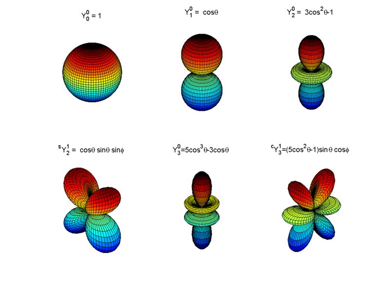
7. A handout entitled Spherical Harmonics examines the solutions to Laplace's equations in spherical coordinates. These solutions possess a radial and angular part; the latter are called the spherical harmonics, Yℓm(θ,φ), where ℓ=0,1,2,3,... and m=-ℓ,-ℓ+1,...,ℓ-1, ℓ. These notes provide a discussion of the properties of the spherical harmonics, along with the famous addition theorem. Two proofs of the addition theorem are given (one in an appendix), and the application to the expansion of the inverse distance function is provided. [PDF | Postscript].
8. A handout entitled The Laplacian of the inverse distance and the Green function provides a derivation of ∇2(1/r)=-4πδ3(r). This result is then applied to solving Poisson's equation. These notes also introduce the concept of the inverse Laplacian and discuss its relation to the Green function. Finally, a derivation of the Green function using Fourier transforms is provided. [PDF | Postscript].
9. A handout entitled The Exclusion-Inclusion principle is extremely useful for certain counting problems. Moreover, it provides a valuable generalization to eq. (3.6) on p. 732 of Boas. In this handout, the inclusion-exclusion principle is derived. This principle is then used to show how to count the number of derangements (i.e. permutations with no fixed points) of n objects. [PDF | Postscript].
10. A handout entitled The normal approximation to the binomial distribution demonstrates that the binomial distribution for successes in n Bernoulli trials with probability for success of p and probability for failure of q=1-p, is very well approximated by the normal distribution when n, np and nq are all very large. [PDF | Postscript].
11. A collection of independent and identically distributed (or iid for short) random variables are a set of random variables with the same probability distribution (or density). These are suitable for modeling independent trials. If x1, x2,..., xn are n iid random variables, then E(xi)=μ and Var(xi)=σ2, for any value of i=1,2,3,...,n. The average of the n random variables is defined by x=(x1+ x2+...+xn)/n. In class, I derived the results E(x)=μ and Var(x) =σ2/n. Details of the derivation are conveniently summarized in the following note by C. Alan Bester from the University of Chicago. [PDF] This note refers to slides that can be found here, although you should be able to confirm each step based on the results obtained in class.
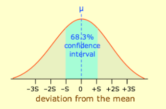
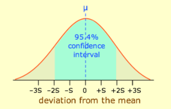
12.The standard deviation of the mean (also called the standard error) provides an estimate of the uncertainty of the experimental determination of the expected value of a random variable. In the case of n measurements, standard error is a factor of n smaller than the standard deviation of the random variable. The latter corresponds to the uncertainty in a single measurement. This distinction is clarified in a class handout entitled The Standard Deviation of the Mean. [PDF | Postscript]
VIII. Free online textbooks
1. A very good source for free mathematical textbooks can be found on FreeScience webpage. I can also provide another useful link to a list of free mathematics textbooks.
2. Sean Mauch (of Caltech) provides a free massive textbook (2321 pages) entitled Introduction to Methods of Applied Mathematics. However, many of the topics of Physics 116C, if treated by Mauch, are in a preliminary status.
3. James Nearing also provides a free textbook entitled Mathematical Tools for Physics. This book treats some of the topics of Physics 116C at a similar level of difficulty.
4. Russel L. Herman has provided notes for a second course in differential equations, covering linear and nonlinear systems and boundary value problems. His monograph is entitled A Second Course in Ordinary Differential Equations: Dynamical Systems and Boundary Value Problems. Of particular interest to Physics 116C are Chapter 6 on Sturm Liouville problems, Chapter 7 on special functions (including Bessel functions and a variety of orthogonal polynomials) and Chapter 8 on Green functions.
5. Kenneth Howell provides links to the chapters of his book entitled Applied Differential Equations, Parts 1--4. Of particular interest to Physics 116C students are the additional chapters that comprise Parts 5--7, which include six chapters on series solutions to differential equations, and four chapters on boundary value problems and Sturm Liouville problems. A consensed version of his chapter on Sturm Liouville problems can be found in his lecture notes for a course in mathematical physics.
6. R.S. Johnson, a professor of applied mathematics at the University of Newcastle upon Tyne has provided, free of charge, a series of mini-books (from the Notebook Series) that cover some of the topics of Physics 116C. These include
- The series solution of second order, ordinary differential equations and special functions
- Sturm-Liouville Theory
- Partial differential equations: classification and canonical forms
7. A textbook entitled Partial Differential Equations for Scientists and Engineers, by Geoffrey Stephenson is available from the following PDF link.
8. A textbook entitled Introduction to Probability, by Charles M. Grinstead and J. Laurie Snell has been generously made available free of charge from the following PDF link, along with PDF solutions to all odd-numbered problems. I especially recommend Chapter 4 for its superb treatment of conditional probability, with applications to the Monty Hall problem, the two-child paradox, and other purported paradoxes that arise in probability theory.
9. Another free textbook on probability entitled Introduction to Probability by Dimitri P. Bertsekas and John N. Tsitsiklis is based on a course taught at MIT. The level of difficulty is appropriate for Physics 116C students. [PDF]
IX. Articles and Books of Interest
1. All the examples of the indicial equations given in Boas possess real roots. But a quadratic equation with real coefficients can also have complex roots. Applying the Frobenius method in the case of complex indicial roots is treated pedagogically in a paper entitled The Frobenius method for complex roots of the indicial equation by Joseph L. Neuringer, International Journal of Mathematical Education in Science and Technology, Volume 9, Issue 1, 1978, pages 71--77. [PDF]
2. The most readable account that I have come across on the Sturm Liouville problem, suitable for Physics 116C students, is Chapter 11 of R. Kent Nagle, Edward B. Saff and Arthur David Snider, Fundamentals of Differential Equations and Boundary Value Problems, 6th Edition (Pearson Education, Inc., Boston, MA, 2012). Unfortunately, this book is too expensive, and there are no previews available either from google or amazon. You may be able to find the most recent or previous editions of this book in the Science and Engineering Library.
3. If you were wondering whether the Laguerre differential equation
can also be solved by factorizing the equation into a product of
first order differential operators and constructing ladder (raising and
lowering) operators, check out the article by H. Fakhri and A. Chenaghlou
entitled
Ladder
operators for the associated Laguerre functions in
J. Phys. A: Math. Gen. 37
(2004) pp. 7499--7507. [PDF]
4. The factorization method for solving differential equations was
made popular by physicists. The method was described in a classic
review paper by L. Infeld and T.E. Hull
entitled The
Factorization Method in Reviews of Modern Physics
23 (1951) pp. 21--68. [PDF]
5. One of the best elementary treatments of partial differential
equations suitable for physicists can be found in a book by Gabriel Barton,
Elements of Green's Functions and Propagation---Potentials,
Diffusion and Waves, published by
Oxford Science Publications in 1989.
Among other things, there is a very clear discussion of
which boundary conditions constitute a well-posed problem.
6. Spherical harmonics play a critical role in computer graphics.
Colorful visual representations of the spherical harmonics provide
added insight into their properties and significance. See for
example, the following two articles:
7. In the Monty Hall problem, there are three doors. Behind one of
them is a brand new car, whereas the other two doors conceal goats.
Monty Hall asks you to choose a door without opening it. Then, he
opens one of the other doors to reveal a goat. At this point,
Monty asks you whether you
wish to switch your choice of doors or to stand pat. Indeed, what is
the probabilty of winning the car if you switch your choice of doors?
When Marylin vos Savant answered this question in the September 9, 1990
issue of Parade magazine, the reader response was overwhelming, many
of whom could not believe her proposed answer that switching resulted
in a probability of 2/3 for winning the car.
Wikipedia
provides an excellent introduction to this problem. For a more
detailed account, read about the history
of the Monty Hall problem and its many variants in this enertaining
book by Jason Rosenhouse entitled
The
Monty Hall Problem: The Remarkable Story of Math's Most
Contentious Brain Teaser (Oxford University Press, Oxford,
UK, 2009).
8. Apparent paradoxes often arise in probability theory. One such
paradox is the called the two-child paradox, which asks for the
probability that a two-child family has two boys given that
one of the children is known to be a boy. Once again,
Wikipedia
provides an excellent introduction to this problem.
I also highly recommend Chapter 4 of the free textbook entitled
Introduction
to Probability, by Charles M. Grinstead and J. Laurie
Snell previously cited in Section XIII of this website. In addition,
check out a fascinating article by Peter Lynch,
The Two-Child Paradox: Dichotomy and
Ambiguity in Irish Mathematical Society Bulletin 67
(2011) pp. 67--73 [PDF].
9. The Monty Hall problem and the two-child paradox can be analyzed
by using conditional probabilites.
Once again, I highly recommend Chapter 4 of
the free textbook entitled Introduction
to Probability, by Charles M. Grinstead and J. Laurie
Snell previously cited in Section XIII of this website.
Another excellent treatment
of these and other well-known puzzles in probability can be found
in an article by Maya Bar-Hillel and Ruma
Falk, Some
teasers concerning conditional probabilities in
Cognition 11 (1982) pp. 109--122
[
PDF].
10. Continuous sample spaces can lead to apparent paradoxical behavior.
I highly recommend Chapter 2 of
the free textbook entitled Introduction
to Probability, by Charles M. Grinstead and J. Laurie
Snell previously cited in Section XIII of this website. This chapter
includes a discussion of Buffon's needle (and the relation of pi to
the probability of where a dropped needle lies). This chapter also
provides a treatment of
Bertrand's paradox, which involves a randomly drawn chord in the unit circle.
11. Finally, I can resist in mentioning
The
Banach-Tarski paradox
which exhibits some very unintuitive phenomena that can
arise in dealing with sets with an uncountable infinite number
of points. For a very readable account, check out the book by
Leonard M. Wapner entitled
The
Pea and the Sun: A Mathematical Paradox (A.K. Peters,
Ltd., Wellesley, MA, 2005). For a slightly more technical
treatment
(which is still accessible to advanced undergraduate students), have a
look at R. French, The Banach-Tarski Theorem, The
Mathematical Intelligencer 10 (1988) 21--28.
12. The law of large numbers and the central limit theorem are treated
at an elementary level in Chapters 8 and 9, respectively of
Introduction
to Probability, by Charles M. Grinstead and J. Laurie
Snell, previously cited in Section XIII of this website.
13. David L. Streiner provides an article entitled
Maintaining Standards: Differences between the Standard Deviation
and Standard Error, and When to Use Each, which should help
illuminate the distinction between the standard deviation and the
standard error (also known as the standard deviation of the mean).
[PDF]
X. Other Web Pages of Interest
1. A superb resource for both the elementary functions and the special functions of mathematical physics is the Handbook of Mathematical Functions by Milton Abramowitz and Irene A. Stegun, which is freely available on-line. The home page for this resource can be found here. There, you will find links to a frames interface of the book. Another scan of the book can be found here. A third independent link to the book can be found here.
2. The NIST Handbook of Mathematical Functions (published by Cambridge University Press), together with its Web counterpart, the NIST Digital Library of Mathematical Functions (DLMF), is the culmination of a project that was conceived in 1996 at the National Institute of Standards and Technology (NIST). The project had two equally important goals: to develop an authoritative replacement for the highly successful Handbook of Mathematical Functions with Formulas, Graphs, and Mathematical Tables, published in 1964 by the National Bureau of Standards (M. Abramowitz and I. A. Stegun, editors); and to disseminate essentially the same information from a public Web site operated by NIST. The new Handbook and DLMF are the work of many hands: editors, associate editors, authors, validators, and numerous technical experts. The NIST Handbook covers the properties of mathematical functions, from elementary trigonometric functions to the multitude of special functions. All of the mathematical information contained in the Handbook is also contained in the DLMF, along with additional features such as more graphics, expanded tables, and higher members of some families of formulas. A PDF copy of the handbook is provided here: [PDF]
3. Another very useful reference for both the elementary functions and the special functions of mathematical physics is An Atlas of Functions (2nd edition) by Keith B. Oldham, Jan Myland and Jerome Spanier, published by Springer Science in 2009. This resource is freely available on-line to students at the University of California at this link.
4. Yet another excellent website for both the elementary functions and the special functions of mathematical physics is the Wolfram Functions site. This site was created with Mathematica and is developed and maintained by Wolfram Research with partial support from the National Science Foundation.
5. One of the classic references to special functions is a three volume set entitled Higher Transcendental Functions (edited by A. Erdelyi), which was compiled in 1953 and is based in part on notes left by Harry Bateman. This was the primary reference for a generation of physicists and applied mathematicians, which is colloquially referred to as the Bateman Manuscripts. Although much of the material goes considerably beyond the level of Physics 116C, this esteemed reference work continues to be a valuable resources for students and professionals. PDF versions of the three volumes are now available free of charge. Check out the three volumes by clicking on the relevant links here: [Volume 1 | Volume 2 | Volume 3].
6. Google is invaluable for searching for mathematical information. For example, if I need the first few Bessel function zeros, I search with google for "Bessel function zeros." The first hit is Bessel function zeros on the Wolfram MathWorld site.
7. Wikipedia provides some good articles on various mathematical topics. For example, a simple exposition on the the law of large numbers can be found here. The Wikipedia treatment of central limit theorem is more technical. What I discussed in class was the classical CLT (or Lindeberg-Levy CLT), which is presented in the first paragraph of the Wikipedia article. However, Wikipedia has another page that illustrates the central limit theorem which is quite illuminating. Check it out at this link.
haber@scipp.ucsc.edu
Last Updated: February 7, 2013