 Click here for the
 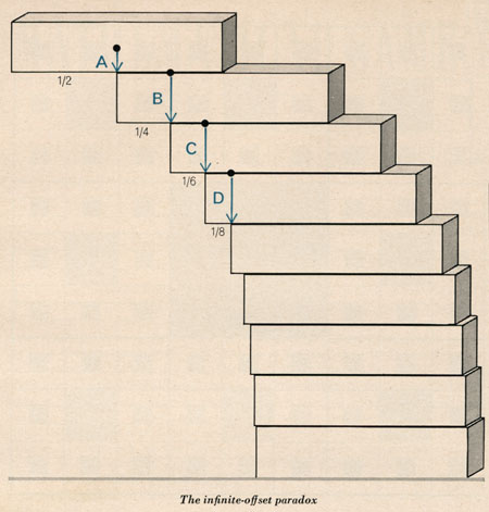 If you stack n bricks on a table,
how far can you make them extend over the edge without toppling?
For bricks of unit length, the answer is given by one-half the
nth harmonic number, i.e. the sum of the series 1/2 + 1/4 + 1/6 + 1/8 +
... + 1/2n.
For more details, click
If you stack n bricks on a table,
how far can you make them extend over the edge without toppling?
For bricks of unit length, the answer is given by one-half the
nth harmonic number, i.e. the sum of the series 1/2 + 1/4 + 1/6 + 1/8 +
... + 1/2n.
For more details, click
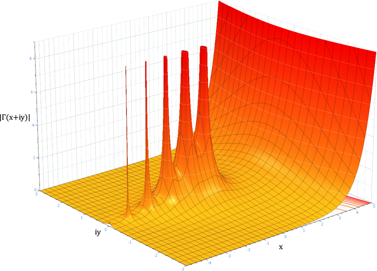
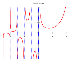 Above, a plot of the gamma function
Γ(x) as a function
of the real variable x. Below, a plot
of the absolute magnitude
of the gamma function |Γ(x+iy)|
plotted in the complex plane. Note the spikes
occur on the negative real axis for
x=0,-1,-2,-3,... where the abolute
value of the gamma function
approaches infinity.
Above, a plot of the gamma function
Γ(x) as a function
of the real variable x. Below, a plot
of the absolute magnitude
of the gamma function |Γ(x+iy)|
plotted in the complex plane. Note the spikes
occur on the negative real axis for
x=0,-1,-2,-3,... where the abolute
value of the gamma function
approaches infinity.
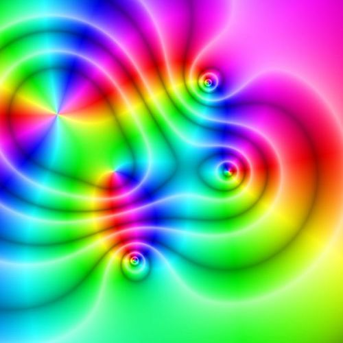
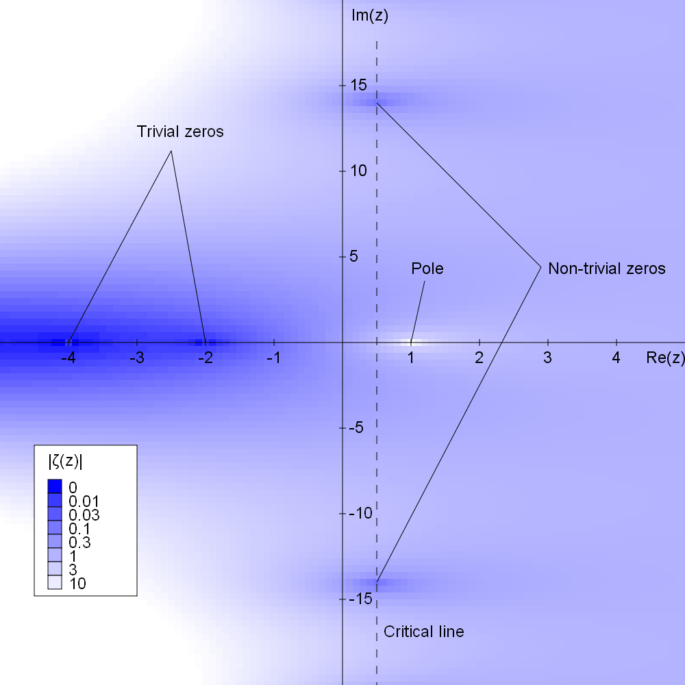 Above is a plot of the absolute value of
the Riemann zeta function |ζ(z)|
plotted in the complex plane (taken from this
Above is a plot of the absolute value of
the Riemann zeta function |ζ(z)|
plotted in the complex plane (taken from this
 The matrix has you. Click
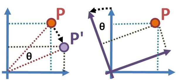 In the active transformation (left), point P moves relative to the
coordinate frame to location P', while the coordinate frame remains
unchanged (in this case, the position of P has rotated clockwise by
angle θ), while in a passive transformation (right), point P is
observed in two different coordinate frames (pictured rotated relative
to one another by angle θ) The coordinates of P' in the active case
are the same as the coordinates of P in the rotated frame in the
passive case if the rotation of P is clockwise and the rotation of the
axes is counterclockwise. (Reference:
In the active transformation (left), point P moves relative to the
coordinate frame to location P', while the coordinate frame remains
unchanged (in this case, the position of P has rotated clockwise by
angle θ), while in a passive transformation (right), point P is
observed in two different coordinate frames (pictured rotated relative
to one another by angle θ) The coordinates of P' in the active case
are the same as the coordinates of P in the rotated frame in the
passive case if the rotation of P is clockwise and the rotation of the
axes is counterclockwise. (Reference:
 The distribution of eigenvalues of a symmetric random matrix with
entries chosen from a standard normal distribution is illustrated
above for a random 5000 x 5000 matrix.
This is an illustration of
The distribution of eigenvalues of a symmetric random matrix with
entries chosen from a standard normal distribution is illustrated
above for a random 5000 x 5000 matrix.
This is an illustration of 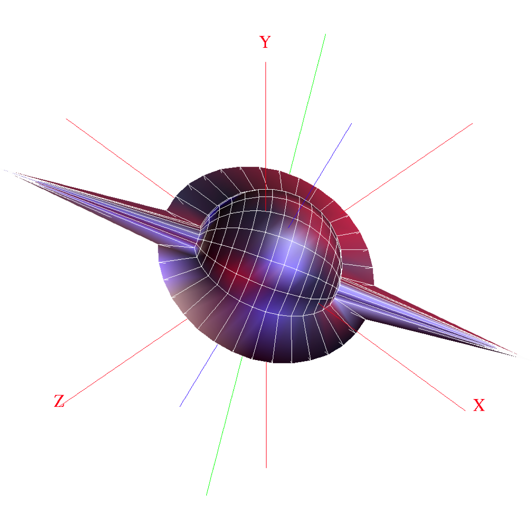 The figure above is a visualization of a symmetric tensor in
three dimensions. The object
in the figure is the sum of a spear, a plate and a sphere. The spear
describes the principal direction of the tensor, where the length is
proportional to the largest eigenvalue. The plate describes the plane
spanned by the eigenvectors corresponding to the two largest
eigenvalues. The sphere, with a radius proportional to the smallest
eigenvalue, shows how isotropic the tensor is. For further details,
check out the following
The figure above is a visualization of a symmetric tensor in
three dimensions. The object
in the figure is the sum of a spear, a plate and a sphere. The spear
describes the principal direction of the tensor, where the length is
proportional to the largest eigenvalue. The plate describes the plane
spanned by the eigenvectors corresponding to the two largest
eigenvalues. The sphere, with a radius proportional to the smallest
eigenvalue, shows how isotropic the tensor is. For further details,
check out the following 
This page contains all class handouts and other items of interest for students of Physics 116A at the University of California, Santa Cruz.
SPECIAL ANNOUNCEMENTS
Final grades for Physics 116A have been assigned. The final exam scores and the final course letter grades are no longer posted. Please stop my office (starting on April 1) to pick up your final exam, any uncollected homeworks, and your final grade.
This website will be kept live for the remainder of the calendar year 2010. Feel free to consult it while you are taking Physics 116B and C.
The distribution of all the final course grades is shown below:
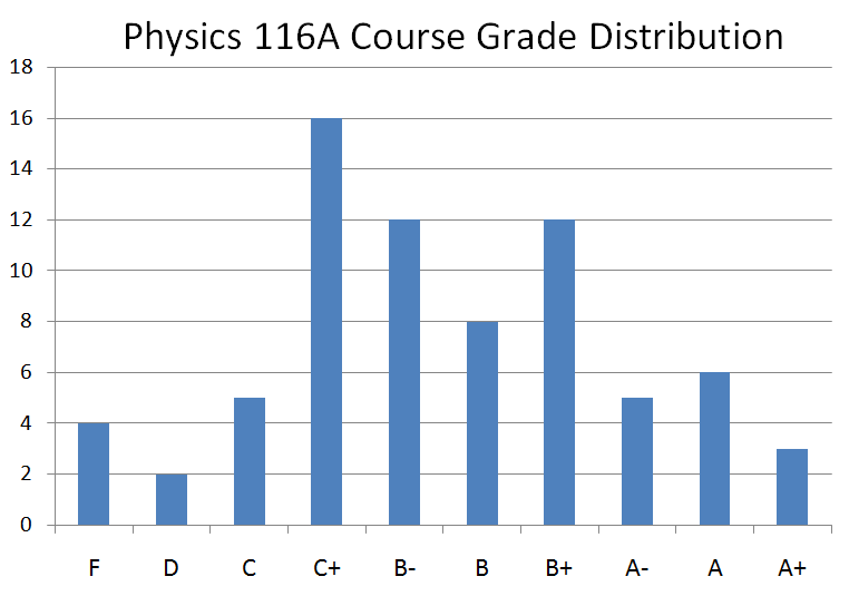
Letter grades are based on the cumulative course average, which
is weighted according to:
homework (9 problem sets with the low score dropped)---40%;
first midterm exam---15%; second first midterm exam---15%; and
the final exam---30%. This cumulative course average is then
converted into a letter grade according to the following
approximate numerical ranges:
A+ (90--100); A (80--90); A- (73--80); B+ (67--73); B (61--67);
B- (55--61); C+ (49--55); C(43--49); D(36--43); F (0--36).
Here is the statistical summary of the distribution of
the cumulative course averages:
mean: 60.6
median: 59
high: 93.9
low : 10.9
Solutions to the final exam (and a link to the final exam statistics)
can be found in Section V on this website.
In addition to the solutions, I provide some bonus material,
which provides some background to problem 4 and explains the
"coincidence" that the same integer sequence appears both in
problems 1 and 4 of the exam (it was no accident!). In section IX,
you can find additional links of interest (cited in the final exam solutions).
Physics 116A: Mathematical Methods in Physics I
I. General Information and Syllabus
The General Information and Syllabus handout is available
in either PDF or Postscript format
[PDF | Postscript]
Some of the information in this handout is reproduced below.
Class Hours
Lectures: Tuesdays and Thursdays, 10--11:45 am, Physical Sciences
Building, Room 110
Required Textbook
Mathematical Methods in the Physical Sciences, by Mary L. Boas
The author keeps track of the latest list of errata for her textbook in the following PDF file.
Course Grading and Requirements
40% Weekly Homework (9 problem sets)
15% First Midterm Exam (Thursday, January 28, 2010)
15% Second Midterm Exam (Tuesday, February 23, 2010)
30% Final Exam (Tuesday, March 16, 2010, 4--7 pm)
Weekly homework assignments will be handed out on a weekly basis, and are due one week later at the beginning of class. The homework problem sets are not optional. You are encouraged to discuss the class material and homework problems with your classmates and to work in groups, but all submitted problems should represent your own work and understanding. In order that homework can be graded efficiently and returned quickly, there will be a 50% penalty for late homework. This penalty may be waived in special circumstances if you see me before the original due date. Homework solutions will be made available two days after the official due date; no late homeworks will be accepted after that.
The two midterm exams and final exams will be held in the same classroom as the lectures. Each midterm will be a one hour exams, and will be followed by a shortened lecture of 45 minutes. The final exam will be three hours long and cover the complete course material. You must take the final exam to pass the course. You will be permitted to consult the class textbook, your own handwritten notes, and any class handout during the exams.
Course Syllabus
The course syllabus is available in either PDF or Postscript format
[PDF | Postscript]
A snapshot of the course lecture schedule appears below.
The dates given below are approximate.
Brief Course Outline for Physics 116A |
||
|---|---|---|
| TOPIC | Lectures dates | Readings |
| Infinite series, power series and asymptotic series | Jan 5, 7, 12 | Boas Chapter 1 | Complex numbers and complex functions | Jan 14, 19, 21 | Boas, Chapter 2 | Special functions defined by integrals | Jan 26, 28, Feb 2, 4 | Boas, Chapter 11 | Matrices, linear algebra and vector spaces | Feb 9, 11, 16, 18, 23 | Boas, Chapter 3 | Eigenvalue problems and matrix diagonalization | Feb 25, March 2, 4 | Boas, Chapter 3 | Tensor Algebra | March 9, 11 | Boas, Chapter 10 |
There will be two midterm exams and one final exam:
- Thursday January 28, 10--11 am Midterm exam #1
- Tuesday February 23, 10--11 am Midterm exam #2
- Tuesday March 16, 4--7 pm Final exam
II. Computer algebra systems
Although the use of computer algebra is not mandatory in this class, it can be a very effective tool for pedagogy. In addition, if used correctly, it can be an invaluable problem solving tool. Two of the best computer algebra systems available are Mathematica and Maple.There are student versions of both Mathematica and Maple available, which sell for the cost of a typical mathematical physics textbook. If you do not wish to invest any money at this time, you can use Mathematica for free at computer labs on campus. For further information click here.
III. Homework Problem Sets and Exams
Problem sets and exams are available in either PDF or Postscript formats.
- Homework Set #1--due: Tuesday January 12, 2010 [PDF | Postscript]
- Homework Set #2--due: Tuesday January 19, 2010 [PDF | Postscript]
- Homework Set #3--due: Tuesday January 26, 2010 [PDF | Postscript]
- Midterm Exam #1---Thursday January 28, 2010 [PDF | Postscript]
- Homework Set #4--due: Thursday February 4, 2010 [PDF | Postscript]
- Homework Set #5--due: Thursday February 11, 2010 [PDF | Postscript]
- Homework Set #6--due: Thursday February 18, 2010 [PDF | Postscript]
- Midterm Exam #2---Tuesday February 23, 2010 [PDF | Postscript]
- Homework Set #7--due: Tuesday March 2, 2010 [PDF | Postscript]
- Homework Set #8--due: Tuesday March 9, 2010 [PDF | Postscript]
- Homework Set #9--due: Monday March 15, 2010 [PDF | Postscript]
- Final Exam---Tuesday March 16, 2010 [PDF | Postscript]
IV. Practice Problems for the Midterm and Final Exams
Practice midterm and final exams can be found here. These should give you some idea as to the format and level of difficulty of the exam.
- Practice Midterm #1 [PDF | Postscript] and their solutions: [PDF | Postscript]
- Additional practice problems #1 [PDF | Postscript] and their solutions: [PDF | Postscript]
- Practice Midterm #2 [PDF | Postscript] and their solutions: [PDF | Postscript]
- Additional practice problems #2 [PDF | Postscript] and their solutions: [PDF | Postscript]
- Practice Final Exam [PDF | Postscript] and their solutions: [PDF | Postscript]
- Additional practice problems #3 [PDF | Postscript] and their solutions: [PDF | Postscript]
V. Solutions to Homework Problem Sets and Exams
The homework set and exam solutions are available in PDF format. Solutions will be posted two days after the homework is due and after the exams have been completed. There is no password required to view the solutions. A link to exam statistics is given for each exam.
- Solution Set #1 [PDF | Postscript] mean score: 91.4 (out of 120 available points)
- Solution Set #2 [PDF | Postscript] mean score: 94.7 (out of 140 available points)
- Solution Set #3 [PDF | Postscript] mean score: 102.2 (out of 140 available points)
- Solutions to Midterm Exam #1 [PDF | Postscript] [exam statistics]
- Solution Set #4 [PDF | Postscript] mean score: 77.1 (out of 120 available points)
- Solution Set #5 [PDF | Postscript] mean score: 70.4 (out of 100 available points)
- Solution Set #6 [PDF | Postscript] mean score: 92.7 (out of 120 available points)
- Solutions to Midterm Exam #2 [PDF | Postscript] [exam statistics]
- Solution Set #7 [PDF | Postscript] mean score: 83.4 (out of 120 available points)
- Solution Set #8 [PDF | Postscript] mean score: 77.0 (out of 120 available points)
- Solution Set #9 [PDF | Postscript] mean score: 68.8 (out of 90 available points)
- Solutions to the Final Exam [PDF | Postscript] [exam statistics]
VI. Other Class Handouts
1. This is a handout
on the alternating series test, with a
clarification on the behavior of series that do not meet all the
conditions of the test.
[PDF | Postscript].
2. The sum of an infinite series of functions is pointwise convergent
over an interval defined by
a < x < b if the sum is convergent at each point in the interval.
It is useful to introduce a stricter notion of convergence called
uniform convergence. Uniformly convergent sums are much better
behaved (see handout number 3 for some examples). All power series
with a radius of convergence R is uniformly convergent over any
closed interval [-r,r], where 0 < r < R. For further details, see the
following class handout , which
distiguishes between these two concepts of a convergent sum of
functions:
[PDF | Postscript].
3. The derivative of an infinite pointwise convergent sum of
functions is not always equal to the sum of the derivatives.
Likewise, the integral of an infinite point-wise convergent sum of
functions is not always equal to the sum of the integrals.
Two explicit
examples of such behavior can be found in this class
handout.
[PDF | Postscript].
4. Taylor series can be used to approximate functions. By summing
over a finite number of terms, it is often possible to obtain
a bound on the error made by replacing the function with the sum of
the first N terms of the Taylor series. (The error will depend on
the point at which the function is evaluated.) One such example
is provided by Theorem 14.4 on p. 35 of Boas. A proof of this theorem
and a simple example are provided in this class
handout.
[PDF | Postscript].
5. A list of Taylor series for some well known functions is provided
in this handout.
The coefficients of the Maclaurin series for tan(x)
and sec(x) depend on the Bernoulli and Euler numbers, respectively.
Some properties of these numbers are presented.
[PDF | Postscript].
6. In this handout,
asymptotic power series are defined and contrasted with
convergent series. The properties of asymptotic series are briefly
summarized. A case example is studied to illuminate the
choice of N such that the sum of the first N terms of the asymptotic
series provides the optimal approximation to the function.
[PDF | Postscript].
7. A complex number can be written in polar form as
z=ei θ, where θ is called the principal value of
the argument of z and is denoted by Arg z. One can also define a
multi-valued argument function as arg z=Arg z+2πn (where n is any
integer). Details of the properties of arg z and Arg z can be found
in this handout.
[PDF | Postscript].
8. A complex logarithm, exponential and power functions do not
possess many of the simple properties associated with the
corresponding real-valued functions. Ignoring this simple fact can
lead to apparent paradoxes. In these highly detailed (and sometime dense)
notes,
I carefully define the complex logarithm, exponential and
power functions, paying careful attention to distinguish between the
multi-valued functions and their single-valued principal value
counterparts.
[PDF | Postscript].
9. The inverse trigonometric and the inverse hyperbolic functions are
multi-valued functions that can be written in terms of the complex
logarithm. In these notes,
I provide a derivation of these expressions.
I also carefully define the (single-valued) principal values of the
inverse trigonometric and the inverse hyperbolic functions, and
compare with the standard conventions for the
real-valued inverse functions.
[PDF | Postscript].
10. One useful application of Euler's formula, ei θ=
cos θ + i sin θ is for summing series that involve the sine
and cosine functions. This technique is especially useful in the
theory of single-slit diffraction. In Physics 5B, I provided some
notes on the derivation of the intensity of the
light due to single slit diffraction. In these notes, the phasor
method is employed, but in the appendix to these notes, I
have provided a derivation
based on Euler's formula. I have reproduced the Physics 5B
handout here.
[PDF | Postscript].
11. In this handout,
I show you how to compute the volume and surface
"area" of an n-dimensional hypersphere. The results depend on the
Gamma function.
[PDF | Postscript].
12. This handout
provides a brief discussion of the properties of the
logarithmic derivative of the Gamma function. In the process, we
learn some fundamental facts about Euler's constant.
[PDF | Postscript].
13. This handout
provides an introduction to the Riemann zeta function
[PDF | Postscript].
Further details and derivations can be found in the following article:
[PDF | Postscript]
14. There is a remarkable connection between the Bernoulli numbers
and the Riemann zeta function evaluated
at the even integers. This handout
provides a "proof" of the formula that exhibits
this relationship. A little
handwaving motivation is used in one step where the mathematical rigor
is lacking. (Euler glossed over the same subtlety!)
[PDF | Postscript].
Further details and derivations can be found in the following article:
[PDF]
15. This handout discusses vector coordinates, matrix elements
and changes of basis. An application to the matrix diagonalization
problem is provided.
[PDF | Postscript].
16. This handout demonstrates a number of basic properties of the
characteristic polynomial of a matrix. These notes discuss
how the coefficients of the characteristic polynomial are related
to the eigenvalues, and provides a general formula for the
coefficients in terms of traces of powers of the matrix.
A proof is given of the Cayley-Hamilton theorem, which states that any
matrix satisfies its own characteristic equation.
[PDF | Postscript].
17. This handout derives an explicit form for the most
general 3x3 rotation matrix, corresponding to a rotation by an angle
θ about an arbitrary axis n. It also provides a very
simple technique for determining the rotation axis and the angle of
rotation given an arbitrary 3x3 rotation matrix. As a bonus,
the relations of
the rotation angle θ and axis n to the Euler angles are
also presented in detail in an appendix to these notes.
[PDF | Postscript].
18.A new derivation of the explicit form for the most
general 3x3 rotation matrix, corresponding to a rotation by an angle
θ about an arbitrary axis n is presented. This elegant
derivation (which is significantly simpler than the one presented
in the previous handout) is based on the methods of tensor algebra.
[PDF | Postscript].
VII. Free online textbooks
1. One of the most useful undergraduate textbooks on mathematical physics is: Mathematical Methods for Physicists, 6th edition, by George B. Arfken and Hans J. Weber. The e-book version is available online in PDF format.
2. Infinite sequences and sums are some of the initial topics studied in a mathematical real analysis course. Such a course provides a sophisticated treatment of concepts first learned in calculus. Here, I provide a free textbook by Brian S. Thomson, Judith B. Bruckner and Andrew M. Bruckner, Elementary Real Analysis, taken from http://www.classicalrealanalysis.com. For this course, I recommend that you peruse Chapters 2, 3, 14 and 16, if you wish to read more about infinite series and power series. These chapters are quite readable for Physics 116A students (even if the rest of the book is somewhat advanced).
3. Sean Mauch (of Caltech) provides a free massive textbook (2321 pages) entitled Introduction to Methods of Applied Mathematics. You may be particularly interested in his treatment of complex numbers. He takes 180 pages to cover the material of Chapter 2 of Boas. I have isolated the two relevant chapters on complex numbers and complex functions to this PDF link. These chapters also provide useful worked out examples.
4. James Nearing also provides a free textbook entitled Mathematical Tools for Physics. This book treats most of the topics of Physics 116A at a similar level of difficulty. Although not as comprehensive as the one by Sean Mauch, you may find some of the presentations enlightening.
5. David A. Santos provides a free textbook on linear algebra which I have uploaded to this website in PDF format. I believe that you will find this quite useful. It covers all the topics of chapters 3 of Boas in greater depth, but at about the same level of sophistication. In addition, it provides many worked out examples.
6. For a more comprehensive (and somewhat more advanced, although very readable) treatment of matrix analysis and linear algebra, check out Matrix Analysis and Applied Linear Algebra by Carl D. Meyer. This modern textbook and solution manual, published by SIAM, has been generously made available for free viewing. Please respect the restrictions to printing and distribution of this material.
VIII. Articles of Interest
1. If the rearrangement of conditionally convergent series strikes your fancy, check out this link for a more in depth discussion of rearranging the alternating harmonic series.
2. There are many proofs that the infinite harmonic series is divergent. Click here for twenty different proofs of this well known theorem. This paper is very elementary and clearly written.
3. The history of pi is fascinating. Check out this review paper by one of the giants in the field of pi research -- Peter Borwein -- in your favorite format: [PDF | Postscript]. Almost anything you wanted to know about pi can be found in this amazing book Pi Unleashed by Jorg Arndt and Christoph Haenel. For a more sophisticated account of pi, I can recommend The Number Pi by Pierre Eymard and Jean-Pierre Lafon.
4. Gregory's series for pi is very slowly converging. Nevertheless, if you sum over the first 500,000 terms, although the 6th digit after the decimal point is wrong, the next ten digits are correct! In fact, only four digits of the first forty are incorrect! The explanation of this curious phenomenon can be understood as a consequence of a certain asymptotic expansion. More details can be found here in an article by J.M. Borwein, P.B. Borwein and K. Dilcher in [PDF] format.
5. The definitions of the principal values of the complex inverse trigonometric and hyperbolic functions involve a number of subtleties. This is especially true for computer programmers who must design their software to produce unique answers. A very nice article that discusses the issues involved and demonstrates how to avoid inconsistencies can be found here: [PDF].
6. Rudolfo Rosales produced an interesting set of notes on branch points and branch cuts for his complex variables course at MIT. You can find these notes here in your favorite format: [PDF | Postscript].
7. Click on the following links to learn more about the gamma function, Euler's constant, the Riemann zeta function and the Bernoulli numbers.
Introduction to the Gamma function
[PDF | Postscript]
The Euler constant
[PDF | Postscript]
Collection of formulae for Euler's constant
[PDF | Postscript]
The Riemann zeta function
[PDF | Postscript]
Introduction to the Bernoulli numbers
[PDF | Postscript]
These articles were found on a web site entitled Numbers, constants and computation, which contains quite a lot of fascinating material. The article on the gamma function covers a number of topics that we were not able to cover in class, including the theorem on the conditions on the uniqueness of the gamma function as the continuous function extrapolation of the factorials of the positive integers. A terrific book on Euler's constant entitled Gamma: Exploring Euler's Constant by Julian Havil is highly recommended.
8. Did you ever wonder how to prove that
 ?
Click
here for
fourteen different proofs of
this result. Proof #6 is basically equivalent to the one that I
presented in class.
If fourteen proofs are too much to handle, try clicking
here for a more modest presentation that
presents six different ways
to sum the series. The latter
presentation is slightly more elementary in style as compared to the former.
?
Click
here for
fourteen different proofs of
this result. Proof #6 is basically equivalent to the one that I
presented in class.
If fourteen proofs are too much to handle, try clicking
here for a more modest presentation that
presents six different ways
to sum the series. The latter
presentation is slightly more elementary in style as compared to the former.
9. A beautifully typeset article (with a pleasing use of colors and photographs) entitled Values of the Riemann zeta function at integers by R.J. Dwilewicz and Jan Minac provides another introduction to some of the mysteries of the Riemann zeta function. In this article, the gamma function, its logarithmic derivative, Euler's constant, and the Bernoulli numbers all play a role in the story. The article is quite readable for the most part (you can ignore the more advanced material that occasionally appears) and definitely worth perusing. It can be found here: [PDF].
10. Boas quotes the following important theorem at the bottom of page 154. A matrix can be diagonalized by a unitary similarity transformation if and only if it is normal, i.e. if the matrix commutes with its hermitian conjugate. For a proof of this result along with a pedagogical treatment of normal matrices written especially for physics students, see Philip A. Macklin, Normal Matrices for Physicists, American Journal of Physics 52, 513--515 (1984). It can be found here: [PDF].
IX. Web Pages of Interest
1. The classic calculus book by R. Courant, Differential and Integral Calculus, Volume 1 is available in html format. Perhaps the chapter most relevant for this course is entitled: "Infinite Series and Other Limiting Processes." The concept of uniform and non-uniform convergence of a series of functions is explained in great detail.
Note: These web pages are best viewed using Internet Explorer. For some reason, some of the symbols are incorrectly rendered when viewed with Firefox.
2. A very good source for free mathematical textbooks can be found on FreeScience webpage. I can also provide another useful link to a list of free mathematics textbooks here.
3. A superb resourece for both the elementary functions and the special functions of mathematical physics is the Handbook of Mathematical Functions by Milton Abramowitz and Irene A. Stegun, which is freely available on-line. The home page for this resource can be found here. There, you will find links to a frames interface of the book. Another scan of the book can be found here.
4. The NIST Handbook of Mathematical Functions (published by Cambridge University Press), together with its Web counterpart, the NIST Digital Library of Mathematical Functions (DLMF), is the culmination of a project that was conceived in 1996 at the National Institute of Standards and Technology (NIST). The project had two equally important goals: to develop an authoritative replacement for the highly successful Handbook of Mathematical Functions with Formulas, Graphs, and Mathematical Tables, published in 1964 by the National Bureau of Standards (M. Abramowitz and I. A. Stegun, editors); and to disseminate essentially the same information from a public Web site operated by NIST. The new Handbook and DLMF are the work of many hands: editors, associate editors, authors, validators, and numerous technical experts. The NIST Handbook covers the properties of mathematical functions, from elementary trigonometric functions to the multitude of special functions. All of the mathematical information contained in the Handbook is also contained in the DLMF, along with additional features such as more graphics, expanded tables, and higher members of some families of formulas.
5. Another excellent website for both the elementary functions and the special functions of mathematical physics is the Wolfram Functions site. This site was created with Mathematica and is developed and maintained by Wolfram Research with partial support from the National Science Foundation.
6. A great source for graphs of mathematical functions, both real-valued and complex-valued, can be found in the Gallery of mathematical functions.
7. Problems 1 and 4 on the final exam provide two independent techniques for solving homogeneous linear difference equations with constant coefficients. The function F(x) in problem 1 is called a generating function for the sequence of integers 0,1,1,3,5,11,21,43,.... To learn more about this technique, I can recommend an amazing book by Herbert S. Wilf, entitled "Generatingfunctionology." The second edition of this book is available for free in pdf format.
These same techniques can also be used to derive a closed-form expression for the nth integer of the Fibonacci sequence (0,1,1,2,3,5,8,13,21,...). The Fibonacci numbers are also intimately connected to the golden ratio (sometimes called the golden mean) which is often denoted by φ=(1+√5)/2. To learn more about the golden ratio, check out this Wikipedia link.
8. Linear transformations have also inspired artists. Check out linear tranformation compositions: a conceptual effort based on the notions of linear algebra, matrices and linear transformations. These compositions evolve from the idea of constantly manipulating a shape endlessly to create a new one. Incessant manipulation and consequent change in shape equals ever-changing, unstable and uncertain characteristics of nature.
haber@scipp.ucsc.edu
Last Updated: June 4, 2010